
- Published on
CH2. The Term Vocabulary and Postings Lists
- Authors

- Name
- seren-wib
Contents
2. The term vocabulary and postings lists
2.1 Documents
Defining what a document is turns out to be a harder question than it seems
In ch1 we assumed we know what a document is and can read it.
In reality, parsing a document is not easy.
- There are three things to decide.
To decide Example format pdf, word, excel, html language English, Korean, French character set UTF-8, EUC-KR. The same bytes are different characters depending on the encoding All three are classification problems.
The alternative is heuristics.
Complications
- One index mixes terms from several languages
- Even a single document mixes them
- What to use as the document unit
- Conclusion: what a document is has no fixed answer; it's a design decision.
2.2 Terms
Problems that come up when turning documents → tokens → terms
| Term | Meaning | Example |
|---|---|---|
| word | The character string exactly as it appears in the text | Windows, U.S.A. |
| term | A normalized word. A group of words treated as the same (equivalence class) | usa (U.S.A., USA) |
| token | One actual occurrence in a document | "the the" → 2 tokens |
| type | Mostly the same as a term. A group of identical tokens | "the the" → 1 type |
General + Non-English
Normalization
- Treat USA = U.S.A
The same word can mean different things in different languages
Tokenization: which tokens to emit
- O'Neill → oneill? o'neill? o + neill?
One word or two
- Whether to split at hyphens, whether to treat words with a space between them as one word
Numbers
- 3/20/91, 20/3/91, Mar 20, 1991 are all the same date
- Old IR systems didn't index numbers, but indexing them is generally useful.
Languages without spaces: where do you split?
Accents and diacritics
English
Case folding: lowercase everything
Stop words: words so common they don't help pick out documents
- things like and, a, by
- Removing them used to be standard, but these days they're kept because phrase queries need them
Other equivalence classes: words that sound the same, or synonyms
Lemmatization
- Inflected or variant forms → the base form listed in a dictionary (lemma)
- A "proper" reduction
- Inflectional: the part of speech stays, only the form changes. cutting → cut
- Derivational: the part of speech changes too. destruction → destroy
Stemming
- A heuristic that roughly chops off word endings
- Roughly imitates what lemmatization tries to do with linguistic knowledge
- Language-specific, and cuts both inflectional and derivational endings
- e.g. automate, automatic, automation → all automat. It's fine if the result isn't a dictionary word.
Lemmatization Stemming Method Find the base form with linguistic knowledge Chop off the ending by rules Result A dictionary word ( be,car)May not be in the dictionary ( automat,poni)Accuracy High Rough Example am, are, is → beautomation → automatPorter algorithm
- The most common algorithm for English stemming
- Conventions + 5 phases applied in order. Each phase has several commands
- Command example: if a word ends in ement and what's left after removing it is longer than 1 character, remove it.
replacement → replac/cement → cement(c is one character, so it isn't removed) - Convention example: within a compound command, pick the rule matching the longest suffix
Rule Example SSES → SS caresses → caress IES → I ponies → poni SS → SS caress → caress S → (removed) cats → cat - caresses matches both SSES and S, but the longer SSES wins → caress (with S it would be caresse)
Comparing three stemmers (part of the same sentence)
Original Porter Lovins Paice analysis analysi analys analys features featur featur feat easily easili eas easy picture pictur pictur pict interpretation interpret interpres interpret - Each stemmer gives different results. Porter cuts the least (Lovins goes as far as the → th, Paice as far as picture → pict)
Does stemming improve effectiveness?
- It depends on the query.
- good case: [sightseeing tour san francisco] → {tour, tours}
- bad case: [operational AND research] (operations research) → Porter maps all of them to oper, so documents with operating or operative also match.
- The gain from grouping is recall (finding more); the cost is precision (also finding wrong ones).
2.3 Skip pointers
Why we need them
- The intersection from ch1 is linear in the list lengths O(x+y)
- Some postings lists have millions of entries, so even linear can be slow.
- Skip pointers let the intersection skip postings that won't end up in the result, so it gets faster
- Two things to decide: where to put skips, and how to skip without making the result wrong
- Basic idea
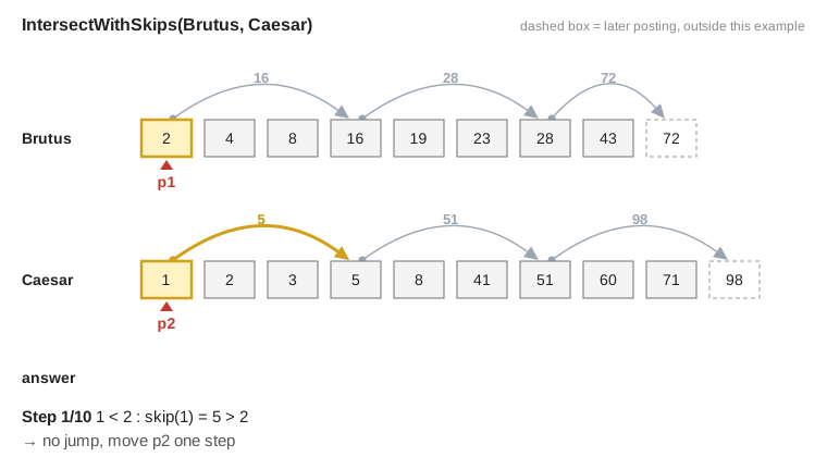
- In the figure: gray arrow = skip pointer, yellow arrow = checked but not taken (target is larger than the other side), green arrow = taken
- e.g. p1 at 16, p2 at 41 → 16 < 41, skip(16) = 28 ≤ 41 → jump to 28. 19 and 23 aren't even compared
- Some postings get one extra pointer that goes several entries ahead.
- Requirement: jump only when the skip target ≤ the other side's docID. Jumping past the other side could miss a match in between.
Algorithm (IntersectWithSkips)
- If the two docIDs are equal: add to answer, advance both by one (same as ch1)
- If not, move the smaller side
- If the smaller side has a skip and the skip target ≤ the other docID: keep taking skips while the condition holds (while, can happen several times in a row)
- Otherwise: advance by one (same as ch1)
- When one side ends, return answer
<=instead of<: jumping to an equal value is a match, so nothing is lost
IntersectWithSkips(p1, p2)
 1 answer <- < >
 2 while p1 != nil and p2 != nil
 3 do if docID(p1) = docID(p2)
 4      then Add(answer, docID(p1))
 5           p1 <- next(p1)
 6           p2 <- next(p2)
 7      else if docID(p1) < docID(p2)
 8           then if hasSkip(p1) and (docID(skip(p1)) <= docID(p2))
 9                  then while hasSkip(p1) and (docID(skip(p1)) <= docID(p2))
10                       do p1 <- skip(p1)
11                  else p1 <- next(p1)
12           else if hasSkip(p2) and (docID(skip(p2)) <= docID(p1))
13                  then while hasSkip(p2) and (docID(skip(p2)) <= docID(p1))
14                       do p2 <- skip(p2)
15                  else p2 <- next(p2)
16 return answer
Where to place skips
How far one skip goes How often it can be used Many skips (narrow spacing) A little Often. But more comparisons and more storage Few skips (wide spacing) A lot Rarely. The target is often larger than the other side - Heuristic: for a list of length P, place √P skips evenly. P = 16 → 4 skips, every 4 entries
- Ignores the distribution of query terms
- Easy for a static index; hard for a dynamic one (documents added or deleted) because the skips have to be placed again
They used to help a lot, but these days CPUs are fast so they don't help much.
2.4 Phrase queries
What phrase queries are and why we need them
- [stanford university] is when the two words must appear next to each other, in that order
- "The inventor Stanford Ovshinsky never went to university" contains both, but shouldn't match.
- A large share of web queries are phrase queries.
- Conclusion: docIDs alone in the postings aren't enough.
- Solutions: biword index, positional index.
Biword index
- Index every pair of adjacent words as a single term.
- e.g. Friends, Romans, Countrymen →
friends romans,romans countrymen - Two-word phrases can be answered right away.
- Longer phrases:
"stanford university palo alto"→"stanford university" AND "university palo" AND "palo alto"- Even if all three are present there's no guarantee the four words are consecutive → false positive → the results have to be filtered again (post-filtering)
- Why it's rarely used: false positives, index blowup
Positional index
- A more efficient alternative to biwords
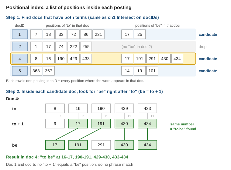
- In the figure: top table = step 1 (docID intersection, one row is one posting), bottom = step 2 (inside doc 4, find to position + 1 = be position)
One posting Normal index docID Positional index docID + the list of positions where it appears in that document to, 993427: 1: <7, 18, 33, 72, 86, 231> 2: <1, 17, 74, 222, 255> 4: <8, 16, 190, 429, 433> 5: <363, 367> be, 178239: 1: <17, 25> 4: <17, 191, 291, 430, 434> 5: <14, 19, 101>to, 993427: 993427 = df /4: <8, 16, ...>= the 8th and 16th words of doc 4 are to- Processing the query
"to be or not to be"- Intersect docIDs (same as ch1) → documents containing both are candidates
- Compare positions inside each candidate: if to is at i, be is at i+1
- Doc 4: to 429, be 430, to 433, be 434 → to be or not to be from 429 → match
Proximity search
- With a positional index, Westlaw's
/kalso works employment /4 place: the two words within 4 words of each other- "Employment agencies that place healthcare workers ..." → hit (1st and 4th: distance 3)
- "Employment agencies that have learned to adapt now place ..." → not a hit (1st and 9th: distance 8)
- The naive way compares every pair of positions of the two words (cross-product) → too slow for common words like the
- It has to return not just the list of documents but also the matching positions (used to build result snippets)
- With a positional index, Westlaw's
PositionalIntersect(p1, p2, k)
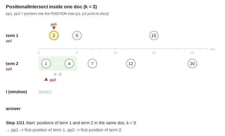
- p1, p2 = pointers to documents (docIDs) / pp1, pp2 = pointers into that document's position lists
- In the figure: green band = pp1 position ± k, l = term 2 positions that came inside the band, answer = (term 1 position, term 2 position) pairs
- The outside is the ch1 Intersect as is; once the same document is found, compare positions inside it
- l = the list of pp2 positions within k of the current pp1 position (used like a window)
- Push pp2 forward and add it to l if within k; stop once it goes too far past pp1
- When pp1 moves forward, drop the values at the front of l that are now farther than k
- For each value left in l, add (docID, pp1 position, pp2 position) to answer
Combination scheme
- Mix biword + positional
- Index only very frequent biwords (Michael Jackson, Britney Spears) as terms → answered right away without comparing positions, so it's fast
- All other phrases use positional intersection
- Williams et al. (2004): faster than positional alone, uses 26% more space
Positional queries are expensive at Google
- Every posting's position list has to be read, and position comparison runs once more after the docID intersection