3. Dictionaries and tolerant retrieval

3.1 Dictionaries

So far we dug into the postings side; this chapter covers the dictionary side.

When a query word comes in, how do we find it in the dictionary quickly?

1. What a dictionary is

   • term vocabulary: the data itself. "Which words exist" (vocabulary = the set of terms, term = one word (no duplicates))
   • dictionary: the data structure that stores that vocabulary

2. Storing it as a fixed-width array

   
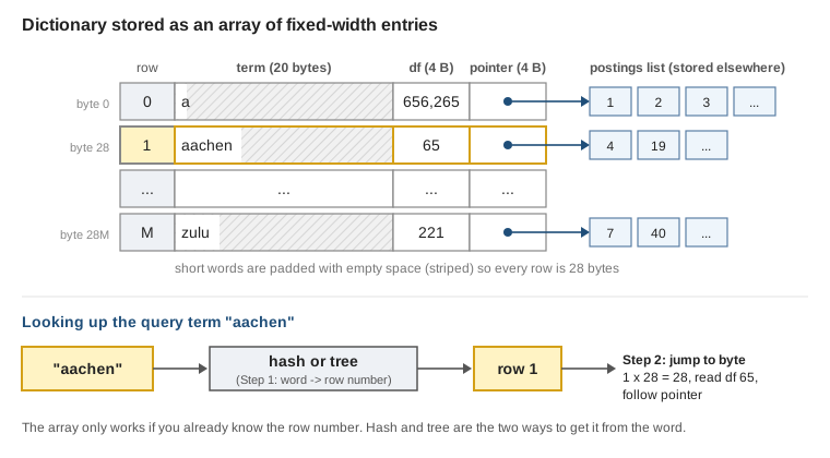
   • Dictionary = an array of rows (one term each). Every row is the same size
   • One row = term (20 bytes) + df (4 bytes) + pointer to the postings list (4 bytes) = 28 bytes, one term per row
   • df: used to AND the shortest lists first (ch1 1.4) / pointer: where the separately stored postings list lives
   • Short words are padded with blanks and still take all 20 bytes (a takes 20 bytes too) → wasteful, covered in ch5 compression
   • Why fixed: row n starts at n × 28 bytes → knowing the row number takes you straight there
   • Problem: queries come in as words, not row numbers → we need something that maps word → row number
   • That something is a hash or a tree (the two kinds of dictionary data structures). The fixed-width array is the storage underneath both, not a third option
   • In the figure: top = the array (stripes = padded blanks), bottom = "aachen" → hash or tree → row 1 → jump to that 28-byte position

3. How to find the array row from a query word

   • hash or tree
   • Differs from one IR system to another. Criteria for choosing:

   Criterion	Hash side	Tree side
   Is the number of terms fixed or growing?	Fixed	Keeps growing (a hash needs rehashing)
   Lookup frequency per key	Mostly exact-word lookups	Prefix and range lookups needed too
   Roughly how many terms?	Size is predictable	Size is hard to predict

4. Hashes

   • Each term is hashed to an integer, and that integer is the array row number
   • So hashing a word takes you straight to its row
   • Pro: faster than a tree. This is O(1)
   • Cons
     1. Can't find similar variants (resume vs résumé); their hash values are completely different
     2. No prefix search (finding every term that starts with automat — the automat from the ch2 stemming example automate, automatic, automation → automat), so no wildcards
     3. When the vocabulary keeps growing and the array fills up (collisions become a problem even before it's full), the array has to be made bigger, which changes every row number, so everything has to be hashed again (rehash)

5. Trees Solves the prefix problem

   • A binary tree is the simplest
   

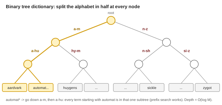
   • Each node splits the alphabet range in half: a-m / n-z → a-hu / hy-m ... → the actual terms are at the leaves

   • In the figure: automat* → a-m → a-hu, and every term starting with automat is gathered below there = prefix search

   • Search is a bit slower than a hash. O(log M), M = vocabulary size

     • But O(log M) only holds for a balanced tree
     • Rebalancing a binary tree is expensive

   • Solution: B-tree

     
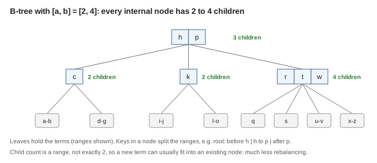
     • Definition: every internal node has a number of children in the interval [a, b]. e.g. [2, 4]
     • In the figure: the root has 3 children, and below it 2, 2, 4 → all within 2 to 4
     • Because the child count is a range rather than exactly 2, a new term can be absorbed inside an existing node → rebalancing happens much less often
     • The keys inside a node (h, p) split the range: before h / h to p / after p

6. Hash vs tree at a glance

   	Hash	Tree (B-tree)
   Lookup speed	O(1), faster	O(log M), a bit slower
   Prefix search (automat*)	X	O
   Finding variants (resume / résumé)	X	Easy, since they're nearby
   When the vocabulary grows	Rehash everything	Rebalance (cheaper with a B-tree)

3.2 Wildcard queries

How do we quickly find the terms matching mon* (monday, month, money) in the dictionary?

Wildcard query → set of matching terms → documents containing any of those terms (OR)

Wildcard query: a query where * stands for any string of characters. e.g. mon* = every document containing a term that starts with mon

1. When * is at the end (mon*)

   • Range search on the B-tree: walk every term t with mon ≤ t < moo
   • This is what 3.1 meant by trees supporting prefix search

2. When * is at the start (*mon)

   • Keep one more B-tree that stores the terms reversed (lemon → nomel)
   • Range search nom ≤ t < non on the reversed tree

3. Processing order

   • Wildcard query → matching set of terms → documents containing any of those terms

4. When * is in the middle (m*nchen)

   • Look up the m* results and the *nchen results separately and intersect them → it works, but it's expensive
   • Alternative: permuterm index

5. Permuterm index

   
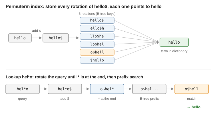
   • Append $ to the end of the term and put every rotation into the B-tree. All of them point to the original term
   • Why rotate * to the end: because the query only works when * is at the end.
   • Relative to $, the left side is the end and the right side is the start
   • hello → hello$, ello$h, llo$he, lo$hel, o$hell, $hello (6 of them)
   • Rotate the query too so * moves to the very end → then it's a prefix search, as in case 1
   • In the figure: top = all 6 rotations linked to hello / bottom = hel*o → o$hel* → key starting with o$hel, o$hell → hello

   Query	Key to look up
   X	X$
   X*	$X*
   *X	X$*
   *X*	X*
   X*Y	Y$X*

   • e.g. hel*o → o$hel*
   • It's called an index but it's really a tree (permuterm tree would be the better name)
   • Downside: the dictionary grows to more than 4 times the size of a regular B-tree (empirical number)

6. k-gram index

   
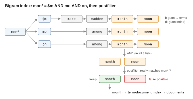
   • k-gram: a sequence of k consecutive characters within a term. 2-gram = bigram
   • $ = word boundary. e.g. april → $a ap pr ri il l$
   • Store k-gram → list of terms containing that k-gram as an inverted index. e.g. (3-gram): etr → beetroot, metric, petrify, retrieval
   • Now there are two kinds of inverted index: term → documents (the original) / k-gram → terms (this one)
   • Handling mon*: $m AND mo AND on → terms starting with mon + false positives like moon
   • Hence postfiltering: check the returned terms against the original query again → look up only the surviving terms in the term-document inverted index
   • In the figure: month and moon appear in all three lists → moon is dropped in postfiltering → only month goes on to the document search

7. k-gram vs permuterm

   	k-gram	permuterm
   Space	Uses less	More than 4 times
   Postfiltering	Needed	Not needed

8. Why Google doesn't fully support wildcards

   • Problem 1: one wildcard expands into many terms → a huge number of Boolean queries to run. [gen* universit*] = (geneva OR genève OR general ...) AND (university OR université ...) → an AND of OR groups, far too expensive
   • Problem 2: users hate typing → if abbreviated queries like [pyth* theo*] are allowed, people will use them a lot → costs go up sharply
   • Google Suggest (autocomplete) mitigates this to some extent

3.3 Edit distance

How to measure, as a number, how far a misspelled query word is from a dictionary term (used for spelling correction in 3.4)

1. Edit distance

   • The minimum number of basic operations needed to turn s1 into s2. e.g. dog → do = 1 (delete g)
   • Levenshtein distance: operations = insert, delete, replace (each costs 1)
   • e.g. dog-do 1 / cat-cart 1 (insert r) / cat-cut 1 (replace a→u) / cat-act 2
   • Damerau-Levenshtein: the 3 above + transposition (swapping two adjacent characters). cat-act = 1 (ca → ac once)

2. Computing it: filling in a matrix

   
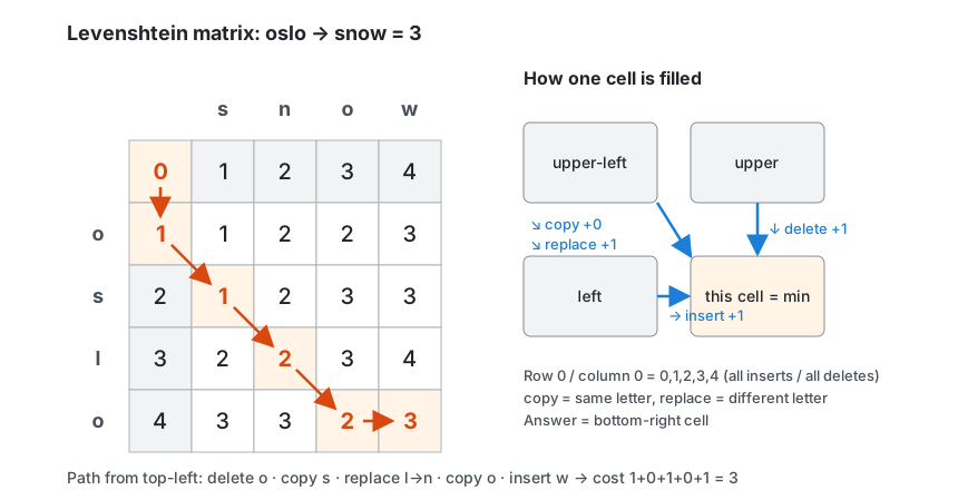
   • Rows = characters of s1, columns = characters of s2. m[i, j] = distance from the first i characters of s1 to the first j characters of s2
   • Row 0 = 0, 1, 2, ... (building j characters from the empty string = j inserts) / column 0 = 0, 1, 2, ... (deleting all i characters = i deletes)
   • One cell = the minimum of three directions
     • ↘ upper-left + 0 (same characters, copy) / + 1 (different, replace)
     • ↓ above + 1 (delete)
     • → left + 1 (insert)
   • Answer = the bottom-right cell
   • In the figure: right = the rule for filling one cell / left = the oslo → snow matrix; following the orange path gives delete o, copy s, replace l→n, copy o, insert w = 3

3. Example: cats → fast = 3

   		f	a	s	t
   	0	1	2	3	4
   c	1	1	2	3	4
   a	2	2	1	2	3
   t	3	3	2	2	2
   s	4	4	3	2	3

   • replace c→f (1), copy a (0), replace t→s (1), replace s→t (1) = 3. Levenshtein has no transposition, so ts → st also costs 2
   • The slide's table splits each cell into four: upper-left = the ↘ value, upper-right = the ↓ value, lower-left = the → value, lower-right = the minimum of the three
   • The sequence of operations is read backwards, climbing up from the bottom-right cell (following whichever direction the minimum came from)

4. Why it's dynamic programming

   • Optimal substructure: the optimal solution as a whole contains optimal solutions to its subproblems. Subproblem = the edit distance between two prefixes
   • Overlapping subsolutions: the same prefix distance is used 3 times (→, ↘, ↓) → store it in the table and don't compute it again

5. Weighted edit distance

   • The cost of an operation depends on which characters are involved. Reflects keyboard typos: m is more often mistyped as n than as q → replacing m→n costs less than m→q
   • Needs a weight matrix as input; when filling the table, add the weight instead of +1

6. Using it for spelling correction

   • List every string within a set (weighted) edit distance of the query word
   • Intersect that with the list of "correct words"
   • Suggest the terms left in the intersection to the user

7. Exercises

   • oslo → snow = 3 (figure)
   • cat → catcat = 3: copy c, a, t + insert c, a, t

3.4 Spelling correction

How to fix a misspelled query word into a correct one

1. Where it's used

   • Correcting documents being indexed / correcting user queries

2. Two approaches

   • isolated word: look at each word on its own and decide whether it's a typo. Misses typos that turn into another correct word. e.g. an asteroid that fell form the sky (form is also a correct word)
   • context-sensitive: also looks at the surrounding words → catches the form/from case above

3. Correcting documents

   • Interactive correction like MS Word is outside the course scope
   • In IR it's mostly used on OCR'd (optical character recognition) documents
   • Basic principle: don't change the documents

4. Query correction: isolated word

   • Premise 1: there is a list of "correct words" to pull correct spellings from
   • Premise 2: we can measure the distance between a typo and a correct word
   • Algorithm: return the correct word closest to the typo. e.g. informaton → information
   • Candidates for the correct-word list
     • The collection's term vocabulary (problem: the collection's documents have typos too, so typos get in as "correct words")
     • A standard dictionary (Webster's, OED) / an industry-specific dictionary (for specialized IR systems) / a weighted collection term vocabulary
   • Ways to measure distance: edit distance (Levenshtein), weighted edit distance, k-gram overlap

5. Correcting with a k-gram index

   • List every k-gram of the query word. e.g. bigrams of bordroom = bo, or, rd, dr, ro, oo, om
   • Fetch the "correct" terms containing those k-grams from the k-gram index
   • Filter by the number of overlapping k-grams (threshold). e.g. only terms that differ by at most 3 k-grams

   bigram	List of terms
   bo	aboard, about, boardroom, border
   or	border, lord, morbid, sordid
   rd	aboard, ardent, boardroom, border

6. Context-sensitive: hit-based

   • e.g. flew form munich
   • Find the nearest correct term for each word: flew → flea, form → from, munich → munch
   • Run every phrase with only one word changed at a time as a query

   Query	Changed word
   flea form munich	flew → flea
   flew from munich	form → from
   flew form munch	munich → munch

   • The phrase with the most hits (number of search results) wins → flew from munich
   • Number of candidates: with 7 for flew, 20 for form, 3 for munich, one at a time = 7 + 20 + 3 = 30 / all combinations = 7 × 20 × 3 = 420
   • Downside: inefficient → look at a collection of queries instead of the documents

7. General issues

   • UI: automatic correction vs suggestion / "Did you mean" only works with a single suggestion; what if there are several? / trade-off between a simple UI and a powerful UI
   • Cost: correction can be expensive → run it only on queries that return few documents instead of on every query? / The guess is that large search engines are efficient enough to run it on every query

8. Exercise: Peter Norvig's spelling corrector

   • NWORDS: frequency of each word in big.txt (words seen for the first time also get 1)
   • edits1(word): every string one edit away = delete, transpose, replace, insert (Damerau-Levenshtein distance 1)
   • known_edits2(word): strings two edits away that are in NWORDS
   • correct(word): candidates = the word itself if it's in the dictionary → otherwise distance 1 → distance 2 → if still nothing, the original word. Returns the candidate with the highest frequency

3.5 Soundex

How to find terms that are spelled differently but sound alike

1. Soundex

   • Finding similar terms by sound (phonetic). Different from 3.3 and 3.4, which are by spelling (orthographic). e.g. chebyshev / tchebyscheff
   • Method: turn every token to be indexed into a 4-character reduced form → turn query terms into the same form → build the index on the reduced forms and search it

2. Algorithm

   1. Keep the first letter

   2. A, E, I, O, U, H, W, Y → 0

   3. Remaining letters → digits

      Letters	Digit
      B, F, P, V	1
      C, G, J, K, Q, S, X, Z	2
      D, T	3
      L	4
      M, N	5
      R	6

   4. Collapse runs of the same digit into one (repeat)

   5. Remove every 0 → pad with trailing 0s and return the first 4 positions = 1 letter + 3 digits

3. Example: HERMAN → H655

   Step	Result
   1. First letter	H
   2·3. Convert ERMAN	06505
   4. Collapse repeats	06505 (none)
   5. Remove 0s	655
   Return	H655

   • HERMANN is also H655: 065055 → 55 becomes 5 in step 4
   • Short ones are padded with 0: LEE → 00 → 0 → nothing left after removal → L000

4. How useful is it

   • Not very, for IR
   • Fine for high-recall tasks where nothing can be missed (e.g. Interpol)
   • Better phonetic matching for IR: Zobel and Dart (1996)

5. ch3 wrap-up (take-away)

   • tolerant retrieval: what to do when query terms and document terms don't match exactly
   • Wildcard queries (3.2) / spelling correction (3.3 and 3.4) / phonetic matching (3.5)