Contents

4. Index construction

4.1 Introduction

How do we build an inverted index for a very large collection → first, the hardware constraints

Hardware basics
- Many IR design decisions are dictated by hardware constraints
- Memory access is much faster than disk (roughly 10×)
- Disk seek = idle time: no data is transferred while the disk head is positioning
- One seek (5 ms) = the time to transfer 250,000 bytes → seeks are overwhelmingly expensive
- One big chunk > many small chunks: disk → memory transfer is fast only if you cut down the number of seeks
- Disk I/O is block-based: whole blocks are read and written, not small pieces. Block size 8KB ~ 256KB
- IR servers: several GB of memory, several TB of disk
- Fault tolerance is expensive → many ordinary machines are cheaper than one expensive machine that never fails (leads into 4.4 distributed indexing)

The RCV1 collection

Shakespeare's collected works are too small → use Reuters RCV1 as the example for scalable index construction
English newswire articles from 1995~1996 (one year). Example: "Extreme conditions create rare Antarctic clouds"

Symbol	Statistic	Value
N	documents	800,000
L	tokens per document	200
M	terms (= word types)	400,000
	bytes per token (incl. spaces/punctuation)	6
	bytes per token (without)	4.5
	bytes per term	7.5
T	non-positional postings	100,000,000

Exercise: how often does a term occur on average = total tokens N × L = 160,000,000 / M 400,000 = 400 times
Exercise: why 4.5 bytes per token vs 7.5 bytes per term = frequent words (the, of, a) are short. The token average counts short words countless times, the term average counts each word only once
Exercise: number of positional postings = one per position = number of tokens = 160,000,000

Exercise: why doesn't this algorithm work for very large collections
- The ch1 approach (load all postings into memory and sort) fails once the postings don't fit in memory → we have to use disk → 4.2 BSBI

4.2 BSBI algorithm

How to sort postings that don't fit in memory by using the disk

Goal: build an inverted index
- dictionary (term) → postings (list of docIDs). Example: Brutus → 1 2 4 11 31 45 173 174
The ch1 approach: sort in memory
- While parsing documents, list (term, docID) pairs → sort by term (then by docID) → group identical terms into postings lists
- Example: Doc 1 I did enact julius caesar ..., Doc 2 so let it be with caesar ... → after sorting: ambitious 2, be 2, brutus 1, brutus 2, capitol 1, caesar 1, caesar 2, ...
Why it fails for large collections
- Documents are parsed one at a time → no term's postings are complete until the last document
- Keep all postings in memory and sort at the end? Not for a large collection → intermediate results must be stored on disk
- Run the same algorithm on disk? No. Sorting on disk needs too many seeks and is slow → we need external sorting
External sorting (RCV1)
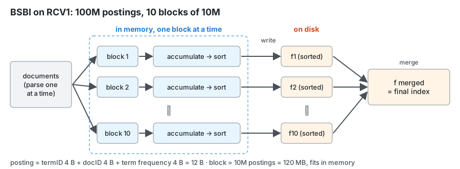
- What to sort: T = 100 million non-positional postings
- One posting = 12 bytes: termID 4 + docID 4 + term frequency 4
- Block = 10 million postings (120MB, fits in memory easily) → RCV1 has 10 blocks
- For each block: (i) accumulate postings (ii) sort in memory (iii) write to disk
- At the end, merge the blocks into one long sorted result
- In the figure: blue dashed box = memory (one block at a time), orange = disk files f1 ~ f10 → merge → final index

Merging two blocks

Each block is already sorted → compare the heads of the two blocks and take the smaller one first (two pointers, like the intersection from ch1)
The blocks as they are: Block 1 = brutus d3, caesar d4, noble d3, with d4 / Block 2 = brutus d2, caesar d1, julius d1, killed d2
Comparison: term first (alphabetical), and if the terms are equal, the smaller docID

Step	Head of Block 1	Head of Block 2	Taken out
1	brutus d3	brutus d2	brutus d2
2	brutus d3	caesar d1	brutus d3
3	caesar d4	caesar d1	caesar d1
4	caesar d4	julius d1	caesar d4
5	noble d3	julius d1	julius d1
6	noble d3	killed d2	killed d2
7	noble d3	(end)	noble d3
8	with d4	(end)	with d4

Merged result = the order things were taken out: brutus d2, brutus d3, caesar d1, caesar d4, julius d1, killed d2, noble d3, with d4

Algorithm
```
BSBIndexConstruction()
n = 0
while (all documents have not been processed)
  n = n + 1
  block = ParseNextBlock()
  BSBI-Invert(block)
  WriteBlockToDisk(block, f_n)
MergeBlocks(f_1, ..., f_n; f_merged)
```
- ParseNextBlock: reads documents and collects one block's worth of (termID, docID) pairs
- BSBI-Invert: sorts the block in memory and groups identical termIDs into postings lists
- WriteBlockToDisk: writes that block's result to disk file f_n
- MergeBlocks: merges f_1 ~ f_n into the final index f_merged

4.3 SPIMI algorithm

A method that removes BSBI's term→termID dictionary problem and doesn't sort either

The problem with BSBI (sort-based)
- Assumption: the dictionary can stay in memory → mapping term → termID needs the dictionary, but the dictionary keeps growing
- What if we use (term, docID) postings instead of termIDs? → intermediate files become huge → it scales, but very slowly
SPIMI (Single-pass in-memory indexing)
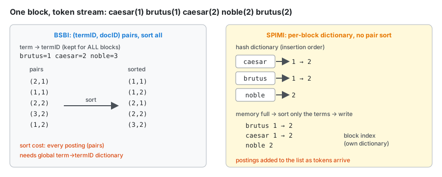
- Key idea 1: build a separate dictionary for each block → no need to keep a term-termID mapping across blocks
- Key idea 2: don't sort. Append each token to its term's postings list as it arrives
- Together these produce one complete inverted index per block → merge them into one big index
- In the figure: left BSBI = sort all termID pairs + one dictionary for all blocks / right SPIMI = append directly to a per-block hash dictionary, sort only the terms when writing

Algorithm

SPIMI-Invert(token_stream)
output_file = NewFile()
dictionary = NewHash()
while (free memory available)
  token = next(token_stream)
  if term(token) not in dictionary
    postings_list = AddToDictionary(dictionary, term(token))
  else
    postings_list = GetPostingsList(dictionary, term(token))
  if full(postings_list)
    postings_list = DoublePostingsList(dictionary, term(token))
  AddToPostingsList(postings_list, docID(token))
sorted_terms = SortTerms(dictionary)
WriteBlockToDisk(sorted_terms, dictionary, output_file)
return output_file

Dictionary = a hash. A new term is added to the dictionary; otherwise its existing postings list is fetched
When a postings list is full, double its size (DoublePostingsList)
Repeat while memory is left → when full, sort only the terms and write the block to disk
Why sort the terms: so the blocks can be read in term order when merging
Merging the blocks is the same as in BSBI

Compression
- Compression makes SPIMI even more efficient: compress terms, compress postings → ch5

BSBI vs SPIMI

	BSBI	SPIMI
Dictionary	keeps one term → termID dictionary going	a new dictionary (hash) per block
Posting form	(termID, docID) pairs	appended directly to each term's postings
Sorting	sorts all pairs	sorts only the terms (once, when writing)
Block result	sorted pairs	a complete inverted index for one block
Merging	merge blocks	same as BSBI

4.4 Distributed indexing

A web-scale index can't be built on one machine → how do we split the work across many failure-prone machines

Why distributed indexing is needed
- Web scale is impossible on one computer → we need a distributed computer cluster
- Individual machines fail often: they slow down or die without warning
- Problem: how do we make use of such an unreliable bunch of machines
Google data centers (2007 estimates)
- Mostly commodity machines instead of expensive servers, spread around the world
- 1 million servers, 3 million processors/cores, 100,000 machines added every quarter
- 200–250 million dollars a year → 10% of the world's computing capacity
Failure calculations
- Probability that all 1000 machines are up = 0.999^1000 ≈ 0.37 (37%) → a system that stops when a single machine dies is unusable
- 1 million servers, each failing once every 3 years → 3 years = 3 × 365 × 24 × 60 = 1,576,800 minutes ÷ 1,000,000 = 1.6 minutes → a machine fails in under 2 minutes
The master and parallel tasks
- master: the machine that directs the whole indexing job. Assumed to be "safe" (never dies)
- Split indexing into many parallel tasks → the master assigns each one to an idle machine
- Two kinds of tasks = two kinds of machines: parser, inverter
- split: a piece (subset of documents) of the document collection. Corresponds to a block in BSBI/SPIMI

Parser and Inverter

	parser	inverter
Receives	one split	one term range (e.g. a-f)
Does	reads documents one by one and emits (term, docID) pairs	collects all (term, docID) pairs (= postings) for that range and sorts
Result	j files, one per term range	the postings lists for that range

term-partition: a range defined by the first letter of the term. Example: a-f, g-p, q-z (j = 3)
segment file: a file a parser writes for each range. j per parser

MapReduce data flow
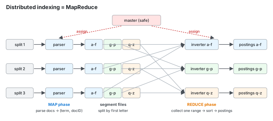
- map = parser: split (group of documents) → (term, docID) pairs → segment files per first-letter range (a-f, g-p, q-z)
- reduce = inverter: collects all segment files for one range and sorts → postings lists
- Order: splits → map phase (parsers) → segment files → reduce phase (inverters) → postings
- In the figure: grey lines = each inverter fetches only its own range's files from every parser

MapReduce

The indexing method we just saw is one instance of MapReduce
MapReduce: a robust and simple framework for distributed computing, so you don't have to write the distribution code yourself
Google's indexing system (around 2002) = many phases, each implemented in MapReduce. Index construction is just one phase
Another phase, for example: converting a term-partitioned index into a document-partitioned index

	term-partitioned	document-partitioned
How it's split	by term range (a-f machine, g-p machine …)	by document group (each machine has a full index of its own documents)
Query handling	machines holding the query terms exchange postings	send to all machines and just merge the results

Exercise: why document-partitioned can be better → even for multi-word queries, long postings lists don't have to move between machines / load doesn't pile up on the machine holding popular terms / if one machine dies, only some documents are missing

Schema of the map and reduce functions

	Input	Output
map	input	list(k, v)
reduce	(k, list(v))	output
indexing map	web collection	list(termID, docID)
indexing reduce	(⟨termID1, list(docID)⟩, ⟨termID2, list(docID)⟩, …)	(postings list1, postings list2, …)

k = termID, v = docID. reduce receives the list of values grouped under the same key

MapReduce worked example

Input: d1: C came, C c'ed. / d2: C died.

Step	Result
map	(C,d2) (died,d2) (C,d1) (came,d1) (C,d1) (c'ed,d1)
group	C → d2, d1, d1 / died → d2 / came → d1 / c'ed → d1
reduce	C → (d1:2, d2:1) / died → (d2:1) / came → (d1:1) / c'ed → (d1:1)

reduce = gather docIDs for each term and count how many times it occurs in each document

Exercise: information exchanged with the master

	What the master gives	What is reported to the master when done
parser	location of its split, how terms are partitioned (a-f, g-p, q-z)	locations of the j segment files it made
inverter	its term range + locations of that range's segment files from all parsers	location of the postings list files it made

4.5 Dynamic indexing

How do we keep the index up to date when documents keep being added, deleted and modified

Why it's needed
- So far we assumed the collection is static
- In reality documents are inserted, deleted and modified → the dictionary and postings lists must keep changing too
The simplest approach: main + aux
- main index: the big index on disk / aux (auxiliary) index: a small in-memory index holding only new documents
- Search: query both and merge the results
- Periodically merge aux into main
- Deletion: don't actually delete; mark a 1 in an invalidation bit-vector → filter the results returned by the index with this vector
Problems with main + aux
- Merges happen often
- Search performance degrades during a merge
Cost of main + aux
- Every time aux (size a) fills up, it's merged into main on disk → all of main is rewritten
- Amount written: a + 2a + 3a + … + na = a · n(n+1)/2 = O(n²) → in terms of total postings T, O(T²) (each posting is rewritten at every merge)
- Example: a = 1, n = 4 → 1 + 2 + 3 + 4 = 10 = 4 × 5 / 2
Logarithmic merge = binary +1
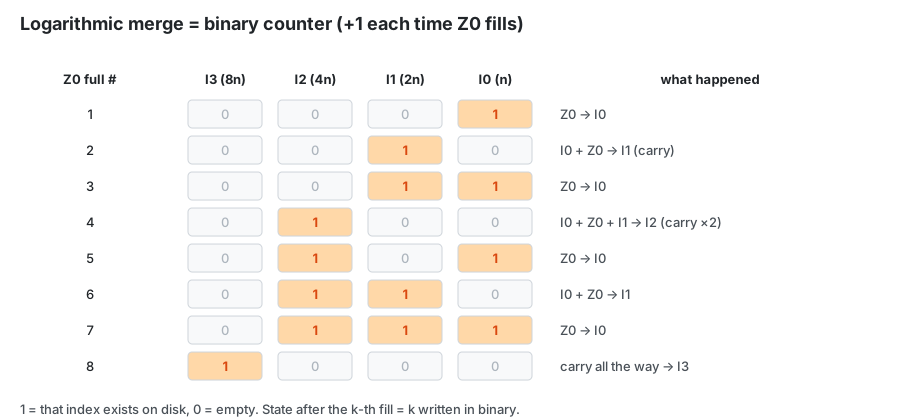
- Spreads (amortizes) the merge cost over time → small impact on the response time users feel
- Each size doubles: Z0 (memory, n) / I0 (n), I1 (2n), I2 (4n), I3 (8n) … (disk)
- When Z0 fills up to n: if I0 is empty → store as I0 / if I0 exists → merge (2n) into I1; if I1 also exists, merge again (4n) into I2 … until an empty slot comes up
- State after the k-th fill = k written in binary (from the right: I0, I1, I2 …). Example: 4th = 100 → only I2, 6th = 110 → I2, I1
- In the figure: orange 1 = that index exists on disk, carry = merge

Algorithm

LMergeAddToken(indexes, Z0, token)
Z0 = Merge(Z0, {token})
if |Z0| = n
  for i = 0 to infinity
    if I_i in indexes
      Z_(i+1) = Merge(I_i, Z_i)
      indexes = indexes - {I_i}
    else
      I_i = Z_i
      indexes = indexes + {I_i}
      break
  Z0 = {}

LogarithmicMerge()
Z0 = {}
indexes = {}
while true
  LMergeAddToken(indexes, Z0, getNextToken())

Add tokens to Z0 one at a time; once Z0 holds n, climb up from i = 0
If Ii exists: merge into Z(i+1) (a temporary index on disk) and remove I_i → go to the next i (carry)
If I_i doesn't exist: Z_i becomes I_i as is → stop
When done, empty Z0 and start receiving again

Cost of logarithmic merge
- Number of indexes = O(log T) → a query only merges O(log T) indexes
- A posting moves up one level each time it's merged → at most log T times → O(T log T) overall
main + aux logarithmic merge
Index construction time O(T²) O(T log T)
Indexes to merge at query time 2 O(log T)
- An order of magnitude more efficient than the aux approach
What large search engines actually do
- Usually a mix of approaches
- Frequent incremental changes
- Build big chunks of the index separately and swap them in whole (rotation, swap in)
- Occasional complete rebuild. Harder the bigger the index; it's unclear whether Google can do a complete rebuild at all
Building positional indexes
- Basically the same problem. The intermediate data structures are just much larger
ch4 take-away
- Two index construction algorithms: BSBI (simple) / SPIMI (more realistic)
- Distributed index construction: MapReduce
- Dynamic index construction: how to keep the index up to date as the collection changes

	main + aux	logarithmic merge
Index construction time	O(T²)	O(T log T)
Indexes to merge at query time	2	O(log T)