
- Published on
CH5. Index Compression
- Authors

- Name
- seren-wib
Contents
5. Index compression
5.1 Compression
Why compress the index → it saves space and also makes things faster
Why compress (in general)
- Saves disk space (saves money)
- Fits more into memory (faster)
- Disk → memory transfer also gets faster: reading compressed data and decompressing it in memory is faster than reading it uncompressed
- Assumption: the decompression algorithm is fast. Everything used in this chapter is fast
Why compress in IR
Target Goal Dictionary Small enough to keep entirely in memory Postings Less disk space, less time reading disk - Large search engines keep a large part of the postings in memory too
lossy vs lossless
- lossy: compression that throws away some information. E.g. case folding, stop word removal, Porter stemming, number elimination (ch2 preprocessing is effectively lossy compression)
- lossless: compression that throws away nothing. Index compression is mostly this
5.2 Term statistics
Before compressing, we need to know roughly how many terms show up (Heaps) and how they are distributed (Zipf)
Reuters RCV1 (same table as ch4 4.1)
Symbol Item Value N Documents 800,000 L Tokens per document 200 M Terms (word types) 400,000 Bytes per token (incl. spaces/punctuation) 6 Bytes per token (without) 4.5 Bytes per term 7.5 T Non-positional postings 100,000,000 Effect of preprocessing on size (Reuters)
- Numbers = % reduction at that step / cumulative %
Step Dictionary (terms) Non-positional postings Positional postings (tokens) Unfiltered 484,494 109,971,179 197,879,290 No numbers 473,723 (−2 / −2) 100,680,242 (−8 / −8) 179,158,204 (−9 / −9) Case folding 391,523 (−17 / −19) 96,969,056 (−3 / −12) 179,158,204 (−0 / −9) 30 stop words 391,493 (−0 / −19) 83,390,443 (−14 / −24) 121,857,825 (−31 / −38) 150 stop words 391,373 (−0 / −19) 67,001,847 (−30 / −39) 94,516,599 (−47 / −52) Stemming 322,383 (−17 / −33) 63,812,300 (−4 / −42) 94,516,599 (−0 / −52) - Exercise: why do the non-positional and positional numbers differ?
- Case folding −3 vs −0, stemming −4 vs −0: if The and the are both in one document, 2 postings (docIDs) merge into 1. But the token count stays the same, so positional doesn't shrink
- Stop words −14 vs −31, −30 vs −47: a stop word appears dozens of times in one document. Non-positional loses only 1 per document, positional loses every occurrence
- Removing stop words barely shrinks the dictionary (removing 30 or 150 is ~0% of the term count)
Heaps' law: estimating vocabulary size
- Is there an upper bound on the vocabulary? No. Words of length 20 alone allow 70²⁰ ≈ 10³⁷ possibilities → as the collection grows, the vocabulary keeps growing
- Heaps' law: an empirical law that predicts the number of terms from the number of tokens in the collection
- M = k · T^b (M = number of terms, T = number of tokens), typically 30 ≤ k ≤ 100, b ≈ 0.5
- A straight line on a log-log plot: log M = b · log T + log k (the simplest relation between collection size and vocabulary size)
- Reuters: log₁₀M = 0.49 · log₁₀T + 1.64 → k = 10^1.64 ≈ 44, b = 0.49
- Example: T = 1,000,020 → 44 × 1,000,020^0.49 ≈ 38,323 (actual 38,365) → a good fit
Heaps' law exercise: find k, b and compute M
- 3,000 terms in the first 10,000 tokens, 30,000 terms in 1,000,000 tokens
- Divide: 30,000 / 3,000 = (1,000,000 / 10,000)^b → 10 = 100^b → b = 0.5
- Substitute: 3,000 = k × 10,000^0.5 = k × 100 → k = 30
- 2 × 10¹⁰ pages × 200 tokens = T = 4 × 10¹² → M = 30 × √(4 × 10¹²) = 30 × 2 × 10⁶ = 60,000,000
- Exercise 1 (keeping typos vs auto-correcting): keeping typos keeps creating new terms, so M gets larger (k or b grows)
Zipf's law: computing frequencies
- Heaps = how big the vocabulary gets / Zipf = how many frequent vs rare terms there are
- Zipf's law: the frequency of the i-th most frequent term is proportional to 1/i. cf_i ∝ 1/i (cf = total occurrences in the collection)
- cf₂ = cf₁ / 2, cf₃ = cf₁ / 3 … e.g. if the is cf₁, of is half of that and and is 1/3
- cf_i = c · i^k (k = −1) → log cf_i = log c − log i → a straight line with slope −1 on a log-log plot (power law)
- On Reuters it doesn't fit the line exactly. What matters is the conclusion: a few frequent terms, a huge number of rare terms
5.3 Dictionary compression
To fit the dictionary in memory, first get rid of the waste in fixed-width slots
Why compress the dictionary
- The dictionary is much smaller than the postings. But it has to stay in memory
- It competes with other programs for memory, devices with little memory such as phones and onboard computers, fast startup time
Fixed-width array (ch3 3.1)
- One row = term 20 + frequency 4 + postings pointer 4 = 28 bytes → (20 + 4 + 4) × 400,000 = 11.2 MB
- Problems
- Most of the term slot is wasted: a 1-letter term also takes 20 bytes
- Words longer than 20 letters don't fit (hydrochlorofluorocarbons, supercalifragilisticexpialidocious)
- Average English term length is about 8 letters → how do we use only about 8 characters per term on average?
Dictionary as a string
- One long string with all terms concatenated + a pointer to each term's start in each row
- Example:
...systilesyzygeticsyzygialsyzygyszaibelyiteszecin.../ the next term's pointer position = the end of the current term - One row = frequency 4 + postings pointer 4 + term pointer 3 + term average 8 bytes (in the string)
- Why the term pointer is 3 bytes: string length 8 × 400,000 = 3,200,000 → log₂(3,200,000) ≈ 21.6 < 24 bits = 3 bytes
- 400,000 × (4 + 4 + 3 + 8) = 7.6 MB (smaller than the fixed-width 11.2 MB)
blocking (k = 4)
- Keep only 1 pointer per 4 terms, and instead prefix each term with a 1-byte length. Example:
7systile9syzygetic8syzygial6syzygy11szaibelyite6szecin - Per block: before, 4 pointers × 3 = 12 bytes → now pointer 3 + lengths 4 × 1 = 7 bytes → 5 bytes saved per block
- Total: 400,000 / 4 blocks × 5 = 0.5 MB → 7.6 → 7.1 MB
- Cost: lookup gets a bit slower
No blocking Blocking (k = 4) How to look up Binary search per term Binary search to the block → linear scan inside block Ex. (8 terms) aid, box, ... all tree nodes [aid box den ex] [job ox pit win], 2 blocks Speed Fast A bit slower - A larger k saves more space but takes longer to scan inside a block
- Keep only 1 pointer per 4 terms, and instead prefix each term with a 1-byte length. Example:
front coding
- front coding: when terms in a block share a prefix, write the prefix only once (they're sorted, so neighbors often share a prefix)
8automata8automate9automatic10automation→8automat*a1◇e2◇ic3◇ion- How to read it:
8automat*a= length 8, the prefix automat ends at*→ automata /1◇e= 1 letter e after the prefix → automate /2◇ic→ automatic /3◇ion→ automation - Exercise: which prefix should be used, and what's the trade-off?
- A long prefix saves more letters per term, but fewer terms share it
- A short prefix is shared by many terms, but saves fewer letters
Dictionary size summary (Reuters, M = 400,000)
Method Computation Size Fixed-width array (20 + 4 + 4) × 400,000 11.2 MB String + term pointers 400,000 × (4 + 4 + 3 + 8) 7.6 MB + blocking (k = 4) 7.6 − 400,000 / 4 × 5 bytes = 7.6 − 0.5 7.1 MB + blocking + front coding 5.9 MB
5.4 Postings compression
Store gaps instead of docIDs, and use a variable length code that spends fewer bits on small gaps
Why compress postings / how many bits per docID
- The postings file is at least 10 times bigger than the dictionary → storing each posting (= one docID) compactly is the key
- 4-byte integer = 32 bits / only as many as needed: log₂ 800,000 ≈ 19.6 → 20 bits
- Goal: far fewer than 20 bits
Storing gaps
- Postings are in ascending docID order → store only the first docID + the difference (gap) from the previous one
- Example: computer 283154, 283159, 283202 → 283154, 5, 43
term docID gap the 283042, 283043, 283044, 283045 1, 1, 1 computer 283047, 283154, 283159, 283202 107, 5, 43 arachnocentric 252000, 500100 252000, 248100 - A frequent term (the) has small gaps / a rare term (arachnocentric) has large ones
Variable length encoding
- An encoding that uses few bits for small gaps and many for large gaps
- Goal: about 20 bits per gap for rare terms like arachnocentric, only a few bits per gap for common terms like the
- Two methods: byte-level VB code / bit-level γ code
VB code (variable byte)
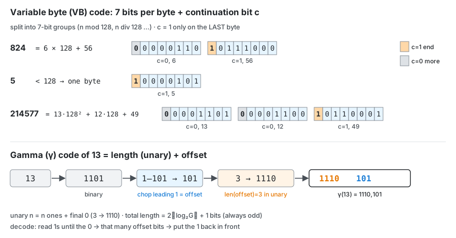
- Widely used in commercial and research systems. Variable length, yet aligned to byte boundaries
- One byte = 1 continuation bit c (first) + 7 bits of number
- Encoding: keep dividing by 128 and fill in the remainders from the back (7 bits each) → only the last byte has c = 1, the rest have c = 0
- Examples: 824 = 6 × 128 + 56 →
00000110 10111000/ 5 →10000101/ 214577 = 13·128² + 12·128 + 49 →00001101 00001100 10110001 - Decoding: n = 128 × n + (7-bit value); when a byte with c = 1 arrives, one number is done → start again with n = 0
- Exercise: 130 = 1 × 128 + 2 →
00000001 10000010 - In the figure: top = VB (orange c = 1 = last byte)
VBEncodeNumber(n) 1 bytes <- < > 2 while true 3 do Prepend(bytes, n mod 128) 4 if n < 128 5 then Break 6 n <- n div 128 7 bytes[Length(bytes)] += 128 8 return bytes VBDecode(bytestream) 1 numbers <- < > 2 n <- 0 3 for i <- 1 to Length(bytestream) 4 do if bytestream[i] < 128 5 then n <- 128 * n + bytestream[i] 6 else n <- 128 * n + (bytestream[i] - 128) 7 Append(numbers, n) 8 n <- 0 9 return numbers- VBEncodeNumber: repeatedly prepend the remainder mod 128 → add 128 to the last byte (= c bit 1)
- VBEncode: run VBEncodeNumber on each number and concatenate
- VBDecode: if below 128 (c = 0), keep accumulating; if 128 or more (c = 1), subtract 128 and accumulate → one number complete
Other variable codes
- Units (alignment) other than bytes are possible: 32 bits (word), 16 bits, 4 bits (nibble)
- With many small gaps, bytes are wasteful → nibbles are better
- There are also word-aligned codes that pack several gaps into one word
Gamma (γ) code
- Bitlevel code: compresses better than VB. The best known is γ
- unary: n → n ones + 0. E.g. 3 →
1110, 40 → 40 ones + 0 - γ = length (unary) + offset
- offset = the binary number with the leading 1 removed: 13 →
1101→101 - length = the number of offset bits in unary: 3 →
1110 - γ(13) =
1110,101
- offset = the binary number with the leading 1 removed: 13 →
- Examples: 1 →
0(no offset) / 2 →10,0/ 3 →10,1/ 4 →110,00/ 9 →1110,001/ 24 →11110,1000/ 511 →111111110,11111111/ 1025 →11111111110,0000000001 - 0 has no γ code (gaps are at least 1, so it doesn't matter)
- Exercise: 130 =
10000010→ offset0000010(7 bits) → length 7 →11111110→ γ(130) =11111110,0000010 - Decoding: count 1s until a 0 (= number of offset bits) → read that many bits → prepend a 1 to get the binary → decimal
- In the figure: bottom = 13 → 1101 → drop the leading 1 → length 3 in unary → concatenate
γ code length
- offset = ⌊log₂G⌋ bits, length = ⌊log₂G⌋ + 1 bits
- Total = 2⌊log₂G⌋ + 1 bits → always odd. E.g. 13 → 2 × 3 + 1 = 7 bits
- Within a factor of 2 of the optimal length log₂G (when the assumption about the gap distribution roughly holds)
Properties of γ codes
- prefix-free: no code is the beginning of another → can be concatenated without separators and still decoded (same for VB)
- Within a factor of 3 of optimal (2 with more assumptions). Holds regardless of the gap distribution
- universal: usable for any distribution
- parameter-free: no parameters to fit
γ vs VB: alignment
- Computers work on 8, 16, 32-bit boundaries → compressing and manipulating at the bit level can be slow
- VB is aligned to byte boundaries, so it can be faster
VB γ Unit Byte Bit Size 116 MB (Reuters) 101 MB (smaller) Speed Fast (aligned) Can be slow Implementation Simple Complex - VB uses a bit more space but is conceptually simpler
Size computation (Reuters)
Data Computation Size (MB) Dictionary, fixed-width 11.2 Dictionary, string + term pointers 7.6 + blocking (k = 4) 7.1 + blocking + front coding 5.9 Collection (text + xml) 3,600 Collection (text only) 960 Term-document incidence matrix 400,000 × 800,000 bits ÷ 8 40,000 Postings, uncompressed (32 bits) 100M × 4 bytes 400 Postings, uncompressed (20 bits) 100M × 2.5 bytes 250 Postings, VB 116 Postings, γ 101 - The index = 10~15% of the collection text (this excludes position and frequency information, so in practice it shrinks less)