6. Scoring, term weighting, the vector space model

6.1 Why ranked retrieval?

Boolean only says match or no match → score each document and show them in order

1. Queries so far have been Boolean

   • A document either matches or it doesn't
   • Good for: experts who know exactly what they want and know the collection / programs that happily consume thousands of results
   • Bad for: most users. They can't write Boolean expressions or don't bother, and don't want to wade through thousands of results (especially in web search)

2. The problem with Boolean search: feast or famine

   • Too many results (200,000) or zero → hard to write a query that returns a manageable number
   • Example: [standard user dlink 650] → 200,000 hits (feast) / [standard user dlink 650 no card found] → 0 hits (famine)
   • ANDing a few more words takes you from 200,000 to 0. Getting a sensible count takes skill

3. Ranked retrieval avoids the problem

   • Even with many results, just show the top 10 → the user isn't overwhelmed
   • Premise: the ranking algorithm has to work (relevant documents on top)

4. Scores are the basis of ranked retrieval

   • Method: assign a score (0~1) to each query-document pair and sort by score. Score = how well the query and document match
   • Score requirements: 0 if no query term appears / higher the more often query terms appear in the document, and the more query terms it contains
   • We look at several scoring methods in turn: Jaccard (6.1) → tf (6.2) → tf-idf (6.3) → cosine (6.4)

5. Computing the Jaccard coefficient

   • jaccard(A, B) = |A ∩ B| / |A ∪ B| (set overlap ratio, 0~1). jaccard(A, A) = 1, 0 if no overlap
   • A and B don't need the same size; the value is always between 0 and 1
   • Example: q "ides of March" = {ides, of, march}, d "Caesar died in March" = {caesar, died, in, march} → ∩ = {march} 1 term, ∪ = 6 terms → 1/6

6. Problems with Jaccard

   • Ignores term frequency: march appearing once or ten times counts the same
   • Ignores that rare terms matter more: the and arachnocentric each count as 1
   • Poor length normalization: later replaced by |A ∩ B| / √|A ∪ B| (cosine, 6.4)

6.2 Term frequency

Put how many times a query term appears in the document into the score

1. Matrices: 0/1 → counts

   • binary incidence matrix: 1 if present, 0 if not (the ch1 matrix). Document = 0/1 vector
   • count matrix: number of occurrences. Example: Anthony in Anthony and Cleopatra = 157. Document = count vector

   	Anthony and Cleopatra	Julius Caesar	The Tempest	Hamlet	Othello	Macbeth
   Anthony	157	73	0	0	0	1
   Brutus	4	157	0	2	0	0
   Caesar	232	227	0	2	1	0
   Calpurnia	0	10	0	0	0	0
   Cleopatra	57	0	0	0	0	0
   mercy	2	0	3	8	5	8
   worser	2	0	1	1	1	5

2. Bag of words

   • bag of words: ignore word order and look only at counts. "John is quicker than Mary" = "Mary is quicker than John"
   • The positional index (ch2 2.4) could tell these apart, so this is a step back
   • Position information comes back later; for now we go with bag of words

3. term frequency (tf)

   • tf_t,d: number of times term t occurs in document d
   • Don't use it raw: tf 10 is more relevant than tf 1, but not 10 times more → relevance doesn't grow in proportion to tf

4. Log-frequency weighting

   • Squash it with a log: w_t,d = 1 + log₁₀ tf_t,d (tf > 0), 0 (tf = 0)

   tf	0	1	2	10	1000
   w	0	1	1.3	2	4

   • tf score = add (1 + log tf_t,d) for every term in both the query and the document. 0 if none

5. Exercise: Jaccard vs tf score

   Query	Document	Jaccard	tf score
   information on cars	all you've ever wanted to know about cars	∩ 1 / ∪ 10 = 0.1	cars 1 → 1
   information on cars	information on trucks, information on planes, information on trains	∩ 2 / ∪ 6 = 0.33	(1 + log 3) × 2 = 2.95
   red cars and red trucks	cops stop red cars more often	∩ 2 / ∪ 8 = 0.25	red 1 + cars 1 = 2

   • Sets count each term once (information 3 times → 1)

6.3 tf-idf weighting

On top of in-document frequency (tf), give more weight to terms that are rare in the collection (idf)

1. In-document frequency vs collection frequency

   • tf = how many times within that document / add how common the term is across the whole collection to the weight too

2. Rare terms vs common terms

   • Rare terms are more informative. Example: a document containing arachnocentric is very likely relevant → high weight
   • Common terms (good, increase, line) are better present than absent, but not a sure sign → positive but low weight
   • We capture this with df

3. Computing idf

   • df_t: the number of documents containing term t. Larger = more common term = less informative (an inverse measure)
   • idf_t = log₁₀ (N / df_t) (N = total number of documents). Larger = more informative term
   • Use a log instead of raw N / df to dampen the effect. Both tf and df use logs
   • Example (N = 1,000,000):

   term	df	idf
   calpurnia	1	6
   animal	100	4
   sunday	1,000	3
   fly	10,000	2
   under	100,000	1
   the	1,000,000	0

   • Shortcut: count the zeros in N / df. 1,000,000 / 100 = 10⁴ → 4

4. Effect of idf on ranking

   • idf only affects ranking when the query has two or more terms (with one term, every document gets multiplied by the same value, so the order doesn't change)
   • Example: "arachnocentric line" → arachnocentric weighs more, line weighs less

5. cf vs df

   • cf_t (collection frequency): number of occurrences of t in the whole collection / df_t: number of documents containing t
   • Example: insurance cf 10440, df 3997 / try cf 10422, df 8760 → similar cf, but insurance is concentrated in fewer documents → insurance is the better search term → weight by df (idf)

   Name	Symbol	Meaning
   term frequency	tf_t,d	occurrences of t in document d
   document frequency	df_t	number of documents containing t
   collection frequency	cf_t	occurrences of t in the whole collection

   • Relations: df ≤ cf (several occurrences in one document still count df as 1) / cf_t = sum of tf_t,d over all documents / tf_t,d ≤ cf_t

6. tf-idf

   • w_t,d = (1 + log tf_t,d) × log (N / df_t) = tf weight × idf weight
   • The best-known weighting scheme in IR. Also written tf.idf, tf x idf
   • Increases with occurrences within the document (tf) and with rarity in the collection (idf)
   • Matrix cells change from counts to real-valued tf-idf: binary → count → weight matrix. Document = real-valued vector (continued in 6.4)

6.4 The vector space model

Treat both documents and queries as tf-idf vectors, and show documents pointing in a similar direction to the query first

1. Documents and queries = vectors

   • Document = real-valued tf-idf vector, one term = one axis (a |V|-dimensional space)
   • Document = a point (vector) in that space
   • Huge number of dimensions (tens of millions for the web), most entries are 0 (sparse)
   • Key idea 1: represent the query as a vector too / key idea 2: rank documents closest (most similar) to the query first
   • The point is to escape Boolean "match or no match" and feast or famine

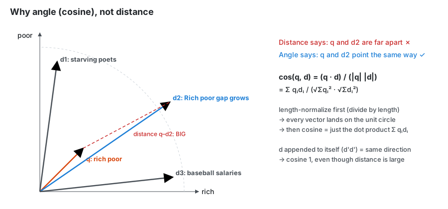
2. Distance doesn't work → angle

   • Euclidean distance is out: vectors of different lengths end up far apart
   • Example: q [rich poor], d2 "Rich poor gap grows" → nearly the same term distribution, yet far apart in distance
   • d' (d appended to itself) has the same content but is far from d. The angle is 0 (maximally similar) → compare by angle
   • Smaller angle = more similar = larger cosine (cosine is decreasing on 0~180°) → ascending angle = descending cosine
   • In the figure: the dotted line (distance) between q and d2 is long, but they point the same way → most similar by cosine

3. Length normalization

   • Divide each value by the vector length (L2 norm, √sum of squares) → length 1 (onto the unit sphere)
   • Long and short documents end up with weights of comparable size
   • d and d' (d twice) become exactly the same vector after normalization

4. Computing cosine

   • cos(q, d) = Σ qᵢdᵢ / (√Σqᵢ² × √Σdᵢ²) (qᵢ, dᵢ = tf-idf weight of term i)
   • = dot product on top, product of the two vector lengths below = cosine of the angle between q and d
   • For normalized vectors, cosine = just multiply and add (dot product)

5. Example: three novels (log tf + cosine normalization, no idf)

   term	SaS tf	PaP tf	WH tf	SaS w	PaP w	WH w	SaS normalized	PaP normalized	WH normalized
   affection	115	58	20	3.06	2.76	2.30	0.789	0.832	0.524
   jealous	10	7	11	2.00	1.85	2.04	0.515	0.555	0.465
   gossip	2	0	6	1.30	0	1.78	0.335	0	0.405
   wuthering	0	0	38	0	0	2.58	0	0	0.588

   • SaS = Sense and Sensibility, PaP = Pride and Prejudice, WH = Wuthering Heights
   • Order: tf → 1 + log tf → compute the length and divide. SaS length = √(3.06² + 2.00² + 1.30²) = √15.05 ≈ 3.88 → 3.06 / 3.88 = 0.789
   • cos(SaS, PaP) = 0.789 × 0.832 + 0.515 × 0.555 + 0.335 × 0 + 0 × 0 ≈ 0.94
   • cos(SaS, WH) ≈ 0.79 / cos(PaP, WH) ≈ 0.69
   • Why SaS-PaP is larger: both weigh affection heavily and have 0 for wuthering. WH has a large wuthering weight, so it points elsewhere

6. The CosineScore algorithm

   CosineScore(q)
   Scores[N] = 0
   for each query term t
     calculate w(t,q), fetch postings list for t
     for each (d, tf(t,d)) in postings list
       Scores[d] += w(t,d) * w(t,q)
   for each d
     Scores[d] = Scores[d] / Length[d]
   return top K of Scores[]
   

   • Go through the postings one term at a time and accumulate (document weight × query weight) into each document's score → divide by document length at the end → top K

7. SMART notation ddd.qqq

   • tf-idf has many variants → written as three letters = tf / df / normalization. First three = document, last three = query
   • Queries and documents often use different weightings

   Position	Letter	Meaning
   tf	n	raw tf
   tf	l	1 + log tf
   tf	a	0.5 + 0.5 × tf / max tf
   tf	b	1 if present, 0 if not
   df	n	not used (1)
   df	t	idf = log (N / df)
   normalization	n	none
   normalization	c	cosine (divide by √sum of squares)

   • The slide table has more: tf L (log ave), df p (prob idf), normalization u (pivoted unique), b (byte size). The default is no weighting
   • lnc.ltn = document: log tf, no idf, cosine normalization / query: log tf, idf, no normalization
   • Is it fine not to apply idf to documents? → the query side applies idf, so the product contains idf once

8. Example: lnc.ltn (N = 1,000,000)

   • Query "best car insurance", document "car insurance auto insurance"

   term	query tf	query w(tf)	df	idf	query weight	doc tf	doc w(tf)	doc normalized	product
   auto	0	0	5000	2.3	0	1	1	0.52	0
   best	1	1	50000	1.3	1.3	0	0	0	0
   car	1	1	10000	2.0	2.0	1	1	0.52	1.04
   insurance	1	1	1000	3.0	3.0	2	1.3	0.68	2.04

   • Query side: 1 + log tf → × idf (no normalization)
   • Document side: 1 + log tf → divide by length √(1² + 0² + 1² + 1.3²) = √3.69 ≈ 1.92 (no idf)
   • Score = sum of products = 0 + 0 + 1.04 + 2.04 = 3.08

9. Summary: ranked retrieval in the vector space model

   1. Represent the query as a tf-idf vector
   2. Represent each document as a tf-idf vector
   3. Compute the cosine between the query vector and each document vector
   4. Rank by cosine
   5. Show the top K (e.g. K = 10)

10. ch6 take-away

    • Why ranking matters: best results first instead of unordered Boolean results (6.1)
    • tf: the core ingredient of ranking (6.2)
    • tf-idf: the best-known traditional ranking scheme (6.3)
    • Vector space model: an important formal model in IR, alongside the Boolean and probabilistic models (6.4)